At this point you have a good command on how to ingest, combine transform, select, filter and visualize datasets. Moreover you are already familiar with time series specific operations.
In this chapter you will learn how to perform advanced transformations on existing dataframes so that they can be further processed by a machine learning pipeline, a statistical technique or just ingested into a dashboarding service.
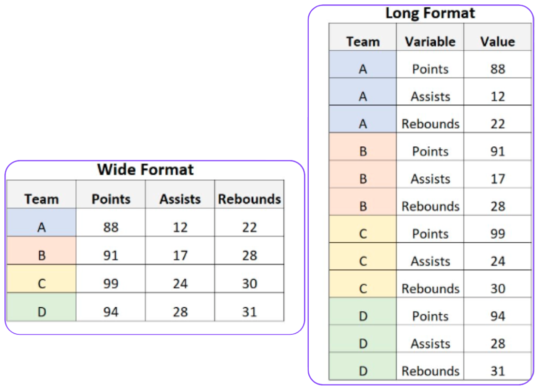
17.1 Long v.s. Wide format DataFrames
In data analysis, long format and wide format refer to two ways of organizing and representing datasets. Each has its use cases, depending on the type of analysis or visualization you need.
Long format
Long format DataFrames have a tidy data structure where each row represents one observation of a single variable or event. Typically, a long format has one identifier column, one variable name column, and one value column, this makes the number of columns fewer compared to a wide format. Since each variable is represented as a separate row, the total number of rows can be larger.
Long format works well when you need to track multiple observations (e.g., stock prices, sensor readings) over time. It is also easier to apply groupby(), aggregation, and pivoting operations on a long format dataset than on their wide format counterparts.
Long format is suitable for multidimensional data as it can handle multiple levels of categorical data (e.g., subject, condition, time) through additional identifier columns.
Wide format
Wide format DataFrames have only one row per entity or observation. Each row represents a single entity (e.g., a person, product, or event) with multiple variables as columns. Wide format has multiple columns, where each variable is stored in a separate column.
Wide format is more compact when you have multiple measurements or variables associated with each entity, making it easy to read and display as a table. Wide format facilitates cross-sectional analysis or summary tables as each row contains all relevant data points for an observation. Wide format is usually the preferred format for machine learning training.
The following figure illustrates the differences between long and wide format.
long v.s. wide formats
Long to Wide Transformation
Pandas offers several methods to transform long format DataFrames to wide format. These methods reshape the data, allowing you to summarize or pivot variables into columns for easier analysis. Main methods are DataFrame.pivot_table() and DataFrame.pivot().
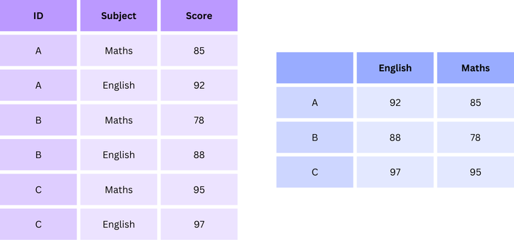
The following example illustrates the use of DataFrame.pivot(). It transforms the dataframe df_long into a wide format, refer to the following figure.
# Use pivot to reshapedf_wide = df_long.pivot(index='ID', columns='Subject', values='Score')df_wide
Subject
English
Maths
ID
A
92
85
B
88
78
C
97
95
The DataFrame.pivot_table() works like DataFrame.pivot() but with the ability to aggregate duplicate entries. It is useful when the data contains duplicate rows for the same index-column pair, and you need to aggregate them.
# Use pivot_table with aggregationdf_wide = df_long.pivot_table(index='ID', columns='Subject', values='Score', aggfunc='mean')df_wide
Subject
English
Maths
ID
A
92.0
85.0
B
88.0
78.0
C
97.0
95.0
Wide to Long Transformation
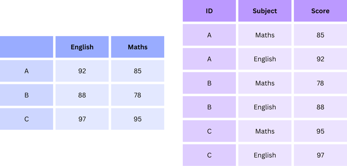
The DataFrame.melt() method is used to reshape data from wide format to long format. It “unpivots” a DataFrame, turning multiple columns into rows, with new columns to hold the variable names and their corresponding values.
The following example transforms a wide format dataframe into its long wide counterpart, refer to the following figure.
# Convert wide format to long format using melt()# id_vars='ID': The ID column remains unchanged, acting as the identifier for each observation.# var_name='Subject': A new column named 'Subject' is created to hold the column names ('Math', 'English') from the original DataFrame.# value_name='Score': A new column named 'Score' is created to store the values from the original columns.df_long = pd.melt(df_wide, id_vars='ID', var_name='Subject', value_name='Score')df_long
ID
Subject
Score
0
A
Math
85
1
B
Math
78
2
C
Math
95
3
A
English
92
4
B
English
88
5
C
English
97
An alternative to reshape DataFrames from wide format to long format is DataFrame.wide_to_long(). It is particularly useful when the column names contain patterns or suffixes. It converts a DataFrame with columns sharing the same prefix (or structure) into a long format by stacking them based on those patterns.
The following example illustrates the use of DataFrame.wide_to_long() to transform a wide format dataframe, this time however we need to interpret the content of some columns in advance.
import pandas as pd# Sample DataFrame in wide formatdf_wide = pd.DataFrame({'ID': [1, 2, 3],'Math_2020': [85, 78, 90],'Math_2021': [88, 82, 92]})df_wide
ID
Math_2020
Math_2021
0
1
85
88
1
2
78
82
2
3
90
92
# Convert wide to long format using wide_to_long()# stubnames='Math': This indicates that we want to reshape columns starting with "Math".# i='ID':The ID column remains as the identifier for each row.# j='Year':A new Year column is created to hold the suffix values (2020, 2021) extracted from the original column names.# sep='_':The separator between the stub name ('Math') and the suffix ('2020', '2021') is _.df_long = pd.wide_to_long(df_wide, stubnames='Math', i='ID', j='Year', sep='_')df_long
Math
ID
Year
1
2020
85
2
2020
78
3
2020
90
1
2021
88
2
2021
82
3
2021
92
17.2 Hierarchical Formats
As data practitioner you need to be prepared to deal with complex formats combining both long and wide formats such as the one shown in the following figure.
hierachical formats
DataFrame flattening, in data science jargon, is the process of transforming a complex, hierarchical structure (like multi-level columns or nested lists within columns) into a simpler, more straightforward structure. Depending on the type of structure you are working with, different methods can be used to “flatten” a DataFrame.
Explode
The DataFrame.explode() method in pandas is used to transform a column in a DataFrame that contains list-like or iterable elements (such as lists, tuples, or sets) into separate rows. This is useful when you have data in a single cell that needs to be expanded across multiple rows for further analysis. The rest of the DataFrame’s columns are repeated for each expanded row.
The following code illustrates the use of DataFrame.explode() to transform the original format into another that can be subsequently converted into a long format by using DataFrame.melt()
Flattening complex dataframe structures can be time consuming and frustrating. For the previous example it is possible to submit the following prompt to your preferred generative AI assistant.
Flatten the following dataframe:
# DataFrame with more complex nested datadf_complex = pd.DataFrame({'Name': ['Alice', 'Bob'],'Scores': [{'Math': 90, 'Science': 85}, {'Math': 75, 'Science': 80}]})
17.3 Handling Categorical Variables
Handling categorical variables in pandas is essential when working with datasets that contain categorical data (i.e., data that can take on a limited number of categories or values). Processing categorical information is relevant in statistical modeling as well as in machine learning (e.g. codification of an image into a discrete set of bits).
The good news is that Pandas provides several tools to work efficiently with categorical variables.
One-Hot Encoding
In Pandas, DataFrame.get_dummies() is a method used for one-hot encoding of categorical variables. It converts categorical columns (with discrete values) into multiple binary columns (0s and 1s) for each unique value in the original column.
The following code performs a one-hot encoding of the variable ‘City’. You will notice that for each city category a new column is created. This format is the one required to train machine learning systems or perform statistical analyses over the data.
Label encoding replaces each category with an integer value. This is useful when you want to preserve the ordinal relationship between categories, or when one-hot encoding would result in too many columns.
The following example converts a categorical variable to a numeric code.
# Convert the 'City' column to categorical typedf['City'] = df['City'].astype('category')# Convert categorical 'City' to numeric codesdf['City_Code'] = df['City'].cat.codesdf
Name
City
City_Code
0
Alice
New York
1
1
Bob
Los Angeles
0
2
Charlie
New York
1
3
Alice
San Francisco
2
4
Bob
Los Angeles
0
Manual Encoding
You can manually map categories to numbers using the Series.map() method. This is especially useful when categories have a specific order or meaning.
Binning, also known as discretisation, is the process of converting continuous numerical variables into discrete categories or intervals. This technique is commonly used in data preprocessing and analysis to group continuous data into “bins” or ranges, making the data easier to interpret, analyze, or use in machine learning models.
Binning is Important in Data Science as it: (1) smooths out noise in data by grouping individual data points into broader categories, (2) reduces the number of unique values, binning makes the data more interpretable and easier to work with, (3) creates new features for machine learning models, especially in algorithms that prefer categorical data (e.g., decision trees).
Pandas provides the pandas.cut() and pandas.qcut() methods for binning.
Pandas cut
The pandas.cut() method is used to bin continuous data into discrete intervals. It is a way of segmenting or sorting data values into bins or categories, which makes it useful for grouping and analyzing continuous data.
The following example bins the column ‘Salary’ into three discrete categories
Pandas.qcut() is used to divide data into equal-sized quantiles. Instead of specifying the exact bin edges, qcut() automatically divides the data into equal-sized groups based on the quantiles.
## we drop the column 'Salary_Level'df_hybrid.drop('Salary_Level',inplace=True,axis=1)## We bin our data using qcut()df_hybrid['Salary_Discretized'] = pd.qcut(df_hybrid['Salary'], q=2, labels=['Low', 'High'])df_hybrid
Name
Age
Salary
Skills
Employed
StartDate
Salary_Discretized
0
Alice
25
70000.50
[Python, SQL]
True
2020-01-01
Low
1
Bob
30
80000.00
[Excel]
False
2021-06-15
Low
2
Charlie
35
90000.75
[Python, Java]
True
2019-03-12
High
17.5 Code Interpretation Challenge
Following please find some examples of python code. Try to understand what the code is trying to accomplish before checking the solution below:
Example: Expanding the Titanic dataset
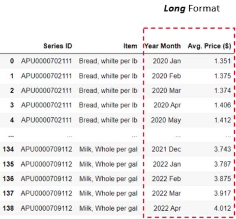
import pandas as pd# URL of the Titanic dataseturl ='https://raw.githubusercontent.com/thousandoaks/Python4DS-I/refs/heads/main/datasets/Titanic-Dataset.csv'# Load the dataset into a DataFramedf = pd.read_csv(url)# Take a random sample of 5 observations from the datasettitanic_sample = df.sample(n=5, random_state=42)# Transform the DataFrame into long formattitanic_long = titanic_sample.melt(id_vars=['PassengerId'], var_name='Attribute', value_name='Value')# Display the transformed DataFramedisplay(titanic_long)
Explanation:
The melt() function is used to transform the sampled DataFrame from wide to long format, id_vars=['PassengerId'] keeps PassengerId as the identifier column. var_name='Attribute' stores the column names in an Attribute column, value_name='Value' stores the corresponding values in a Value column.
PassengerId
Attribute
Value
0
710
Survived
1
1
440
Survived
0
2
841
Survived
0
3
721
Survived
1
4
40
Survived
1
5
710
Pclass
3
6
440
Pclass
2
7
841
Pclass
3
8
721
Pclass
2
9
40
Pclass
3
10
710
Name
Moubarek, Master. Halim Gonios ("William George")
11
440
Name
Kvillner, Mr. Johan Henrik Johannesson
12
841
Name
Alhomaki, Mr. Ilmari Rudolf
13
721
Name
Harper, Miss. Annie Jessie "Nina"
14
40
Name
Nicola-Yarred, Miss. Jamila
15
710
Sex
male
16
440
Sex
male
17
841
Sex
male
18
721
Sex
female
19
40
Sex
female
20
710
Age
NaN
21
440
Age
31.0
22
841
Age
20.0
23
721
Age
6.0
24
40
Age
14.0
25
710
SibSp
1
26
440
SibSp
0
27
841
SibSp
0
28
721
SibSp
0
29
40
SibSp
1
30
710
Parch
1
31
440
Parch
0
32
841
Parch
0
33
721
Parch
1
34
40
Parch
0
35
710
Ticket
2661
36
440
Ticket
C.A. 18723
37
841
Ticket
SOTON/O2 3101287
38
721
Ticket
248727
39
40
Ticket
2651
40
710
Fare
15.2458
41
440
Fare
10.5
42
841
Fare
7.925
43
721
Fare
33.0
44
40
Fare
11.2417
45
710
Cabin
NaN
46
440
Cabin
NaN
47
841
Cabin
NaN
48
721
Cabin
NaN
49
40
Cabin
NaN
50
710
Embarked
C
51
440
Embarked
S
52
841
Embarked
S
53
721
Embarked
S
54
40
Embarked
C
Example: One Hot encoding of the Titanic dataset
import pandas as pd# URL of the Titanic dataseturl ='https://raw.githubusercontent.com/thousandoaks/Python4DS-I/refs/heads/main/datasets/Titanic-Dataset.csv'# Load the dataset into a DataFramedf = pd.read_csv(url)df_reduced=df[['PassengerId','Survived','Name','Pclass']]# Perform one-hot encoding on the 'Pclass' columntitanic_encoded = pd.get_dummies(df_reduced, columns=['Pclass'], prefix='Class')# Display the resulting DataFramedisplay(titanic_encoded.head())
Explanation:
The code applies one-hot encoding to the Pclass column using pd.get_dummies() to create binary columns for each class, and displays the transformed DataFrame.
PassengerId
Survived
Name
Class_1
Class_2
Class_3
0
1
0
Braund, Mr. Owen Harris
False
False
True
1
2
1
Cumings, Mrs. John Bradley (Florence Briggs Th...
True
False
False
2
3
1
Heikkinen, Miss. Laina
False
False
True
3
4
1
Futrelle, Mrs. Jacques Heath (Lily May Peel)
True
False
False
4
5
0
Allen, Mr. William Henry
False
False
True
Example: Binning the Titanic dataset
import pandas as pd# URL of the Titanic dataseturl ='https://raw.githubusercontent.com/thousandoaks/Python4DS-I/refs/heads/main/datasets/Titanic-Dataset.csv'# Load the dataset into a DataFramedf = pd.read_csv(url)# Define age bins and labelsage_bins = [0, 10, 20, 40, 60, 100]age_labels = ['0-10', '10-20', '20-40', '40-60', '60-100']# Create a new column 'AgeGroup' with binned age valuesdf['AgeGroup'] = pd.cut(df['Age'], bins=age_bins, labels=age_labels, right=False)# Display the updated DataFrame with the new 'AgeGroup' columnprint(df[['Name','Age', 'AgeGroup']].head(10))
Explanation:
The code applies one-hot encoding to the Pclass column using pd.get_dummies() to create binary columns for each class, and displays the transformed DataFrame.
                                                Name   Age AgeGroup
0                            Braund, Mr. Owen Harris  22.0    20-40
1  Cumings, Mrs. John Bradley (Florence Briggs Th...  38.0    20-40
2                             Heikkinen, Miss. Laina  26.0    20-40
3       Futrelle, Mrs. Jacques Heath (Lily May Peel)  35.0    20-40
4                           Allen, Mr. William Henry  35.0    20-40
5                                   Moran, Mr. James   NaN      NaN
6                            McCarthy, Mr. Timothy J  54.0    40-60
7                     Palsson, Master. Gosta Leonard   2.0     0-10
8  Johnson, Mrs. Oscar W (Elisabeth Vilhelmina Berg)  27.0    20-40
9                Nasser, Mrs. Nicholas (Adele Achem)  14.0    10-20
17.6 Advanced Data Transformation in Practice
First Example (Digital Marketing)
Let’s have a look at the following Jupyter Notebook. This notebook illustrates how to process real information from customer’s preferences regarding digital streaming content. This kind of transformations are required in machine learning contexts, for instance to train a recommender system.
Second Example (Healthcare)
The following notebook Jupyter Notebook illustrates some data transformations performed over a healthcare dataset for the purposes of operational benchmarking and visualization.
Third Example (Retail)
The following notebook Jupyter Notebook illustrates some data transformations performed over a retail dataset for the purposes of operational benchmarking and visualization.
17.7 Conclusion
This chapter delves into advanced data transformations, essential for preparing datasets for machine learning pipelines, statistical analyses, or dashboard integration. It contrasts long and wide data formats, explaining that long formats, with fewer columns but more rows, are ideal for multidimensional data and operations like aggregation and pivoting. Wide formats, on the other hand, are compact and better suited for machine learning models and summary analyses. Methods like DataFrame.pivot() and DataFrame.pivot_table() convert long data to wide formats, while methods like DataFrame.melt() and DataFrame.wide_to_long() reverse this transformation. Hierarchical and complex structures, such as nested or multi-level columns, can be flattened using DataFrame.explode(), apply(pd.Series), or related methods for streamlined processing.
The chapter also covers handling categorical variables through encoding techniques. One-hot encoding creates binary columns for each category, while label encoding assigns numeric codes to categories. Manual mapping is also explored for custom encodings. It introduces binning, which discretises continuous variables into categorical intervals using DataFrame.cut() for defined bins or DataFrame.qcut() for quantile-based bins, aiding in noise reduction and feature creation. Practical examples from digital marketing, healthcare, and retail highlight these techniques’ applications, illustrating their role in transforming raw data into formats ready for advanced analysis or modeling.
17.8 Further Readings
For those of you in need of additional, more advanced, topics please refer to the following references: